Figure 9. Important Haskell classes
In Star Trek, Spock had a special talent of connecting with a character with what he called the mind meld. Haskell enthusiasts often claim such a connection to their language. For many of them, the language feature that engenders the most respect is the type system. After spending so much time with the language, I can easily see why this is true. The type system is flexible and rich enough to infer most of my intent, staying out of my way unless I need it. I also get a sanity check as I build my functions, especially the abstract ones that compose functions.
Haskell’s type system is one of its strongest features. It allows type inference, so programmers do not have heavier responsibilities. It is also robust enough to catch even subtle programming errors. It is polymorphic, meaning you can treat different forms of the same type the same. In this section, we’ll look at a few examples of types and then build some of our own types.
Let’s review what you’ve learned so far with some basic types. First, we’ll turn on the type option in the shell:
Prelude> :set +t
|
Now, we’ll see the types that each statement returns. Try some characters and strings:
Prelude> 'c'
|
|
'c'
|
|
it :: Char
|
|
Prelude> "abc"
|
|
"abc"
|
|
it :: [Char]
|
|
Prelude> ['a', 'b', 'c']
|
|
"abc"
|
|
it :: [Char]
|
it always gives you the value of the last thing you typed, and you can read :: as is of type. To Haskell, a character is a primitive type. A string is an array of characters. It doesn’t matter how you represent the array of characters, with an array or with the double quotes. To Haskell, the values are the same:
Prelude> "abc" == ['a', 'b', 'c']
|
|
True
|
There are a few other primitive types, like this:
Prelude> True
|
|
True
|
|
it :: Bool
|
|
Prelude> False
|
|
False
|
|
it :: Bool
|
As we dig deeper into typing, these ideas will help us see what’s really going on. Let’s define some of our own types.
We can define our own data types with the data keyword. The simplest of type declarations uses a finite list of values. Boolean, for example, would be defined like this:
data Boolean = True | False
|
That means that the type Boolean will have a single value, either True or False. We can define our own types in the same way. Consider this simplified deck of cards, with two suits and five ranks:
| haskell/cards.hs | |
module Main where
|
|
data Suit = Spades | Hearts
|
|
data Rank = Ten | Jack | Queen | King | Ace
|
|
In this example, Suit and Rank are type constructors. We used data to build a new user-defined type. You can load the module like this:
*Main> :load cards.hs
|
|
[1 of 1] Compiling Main ( cards.hs, interpreted )
|
|
Ok, modules loaded: Main.
|
|
*Main> Hearts
|
|
|
|
<interactive>:1:0:
|
|
No instance for (Show Suit)
|
|
arising from a use of `print' at <interactive>:1:0-5
|
Argh! What happened? Haskell is basically telling us that the console is trying to show these values but doesn’t know how. There’s a shorthand way to derive the show function as you declare user-defined data types. It works like this:
| haskell/cards-with-show.hs | |
module Main where
|
|
data Suit = Spades | Hearts deriving (Show)
|
|
data Rank = Ten | Jack | Queen | King | Ace deriving (Show)
|
|
type Card = (Rank, Suit)
|
|
type Hand = [Card]
|
|
Notice we added a few alias types to our system. A Card is a tuple with a rank and a suit, and a Hand is a list of cards. We can use these types to build new functions:
value :: Rank -> Integer
|
|
value Ten = 1
|
|
value Jack = 2
|
|
value Queen = 3
|
|
value King = 4
|
|
value Ace = 5
|
|
|
|
cardValue :: Card -> Integer
|
|
cardValue (rank, suit) = value rank
|
For any card game, we need to be able to assign the ranks of a card. That’s easy. The suit really doesn’t play a role. We simply define a function that computes the value of a Rank and then another that computes a cardValue. Here’s the function in action:
*Main> :load cards-with-show.hs
|
|
[1 of 1] Compiling Main ( cards-with-show.hs, interpreted )
|
|
Ok, modules loaded: Main.
|
|
*Main> cardValue (Ten, Hearts)
|
|
1
|
We’re working with a complex tuple of user-defined types. The type system keeps our intentions clear, so it’s easier to reason about what’s happening.
Earlier, you saw a few function types. Let’s look at a simple function:
backwards [] = []
|
|
backwards (h:t) = backwards t ++ [h]
|
We could add a type to that function that looks like this:
backwards :: Hand -> Hand
|
|
...
|
That would restrict the backwards function to working with only one kind of list, a list of cards. What we really want is this:
backwards :: [a] -> [a]
|
|
backwards [] = []
|
|
backwards (h:t) = backwards t ++ [h]
|
Now, the function is polymorphic. [a] means we can use a list of any type. It means that we can define a function that takes a list of some type a and returns a list of that same type a. With [a] -> [a], we’ve built a template of types that will work with our function. Further, we’ve told the compiler that if you start with a list of Integers, this function will return a list of Integers. Haskell now has enough information to keep you honest.
Let’s build a polymorphic data type. Here’s one that builds a three-tuple having three points of the same type:
| haskell/triplet.hs | |
module Main where
|
|
data Triplet a = Trio a a a deriving (Show)
|
|
On the left side we have data Triplet a. In this instance, a is a type variable. So now, any three-tuple with elements of the same type will be of type Triplet a. Take a look:
*Main> :load triplet.hs
|
|
[1 of 1] Compiling Main ( triplet.hs, interpreted )
|
|
Ok, modules loaded: Main.
|
|
*Main> :t Trio 'a' 'b' 'c'
|
|
Trio 'a' 'b' 'c' :: Triplet Char
|
I used the data constructor
Trio to build a three-tuple. We’ll talk more about the data constructors in the next section. Based on our type declaration, the result was a Triplet a, or more specifically, a Triplet char and will satisfy any function that requires a Triplet a. We’ve built a whole template of types, describing any three elements whose type is the same.
You can also have types that are recursive. For example, think about a tree. You can do this in several ways, but in our tree, the values are on the leaf nodes. A node, then, is either a leaf or a list of trees. We could describe the tree like this:
| haskell/tree.hs | |
module Main where
|
|
data Tree a = Children [Tree a] | Leaf a deriving (Show)
|
|
So, we have one type constructor, Tree. We also have two data constructors, Children and Leaf. We can use all of those together to represent trees, like this:
Prelude> :load tree.hs
|
|
[1 of 1] Compiling Main ( tree.hs, interpreted )
|
|
Ok, modules loaded: Main.
|
|
*Main> let leaf = Leaf 1
|
|
*Main> leaf
|
|
Leaf 1
|
First, we build a tree having a single leaf. We assign the new leaf to a variable. The only job of the data constructor Leaf is to hold the values together with the type. We can access each piece through pattern matching, like this:
*Main> let (Leaf value) = leaf
|
|
*Main> value
|
|
1
|
Let’s build some more complex trees.
*Main> Children[Leaf 1, Leaf 2]
|
|
Children [Leaf 1,Leaf 2]
|
|
*Main> let tree = Children[Leaf 1, Children [Leaf 2, Leaf 3]]
|
|
*Main> tree
|
|
Children [Leaf 1,Children [Leaf 2,Leaf 3]]
|
We build a tree with two children, each one being a leaf. Next, we build a tree with two nodes, a leaf and a right tree. Once again, we can use pattern matching to pick off each piece. We can get more complex from there. The definition is recursive, so we can go as deep as we need through let and pattern matching.
*Main> let (Children ch) = tree
|
|
*Main> ch
|
|
[Leaf 1,Children [Leaf 2,Leaf 3]]
|
|
*Main> let (fst:tail) = ch
|
|
*Main> fst
|
|
Leaf 1
|
We can clearly see the intent of the designer of the type system, and we can peel off the pieces that we need to do the job. This design strategy obviously comes with an overhead, but as you dive into deeper abstractions, sometimes the extra overhead is worth the hassles. In this case, the type system allows us to attach functions to each specific type constructor. Let’s look at a function to determine the depth of a tree:
depth (Leaf _) = 1
|
|
depth (Children c) = 1 + maximum (map depth c)
|
The first pattern in our function is simple. If it’s a leaf, regardless of the content of the leaf, the depth of the tree is one.
The next pattern is a little more complicated. If we call depth on Children, we add one to maximum (map depth c). The function maximum computes the maximum element in an array, and you’ve seen that map depth c will compute a list of the depths of all the children. In this case, you can see how we use the data constructors to help us match the exact pieces of the data structure that will help us do the job.
So far, we’ve been through the type system and how it works in a couple of areas. We’ve built user-defined type constructors and got templates that would allow us to define data types and declare functions that would work with them. Haskell has one more important concept related to types, and it’s a big one. The concept is called the class, but be careful. It’s not an object-oriented class, because there’s no data involved. In Haskell, classes let us carefully control polymorphism and overloading.
For example, you can’t add two booleans together, but you can add two numbers together. Haskell allows classes for this purpose. Specifically, a class defines which operations can work on which inputs. Think of it like a Clojure protocol.
Here’s how it works. A class provides some function signatures. A type is an instance of a class if it supports all those functions. For example, in the Haskell library, there’s a class called Eq.
Here’s what it looks like:
class Eq a where
|
|
(==), (/=) :: a -> a -> Bool
|
|
|
|
-- Minimal complete definition:
|
|
-- (==) or (/=)
|
|
x /= y = not (x == y)
|
|
x == y = not (x /= y)
|
So, a type is an instance of Eq if it supports both == and /=. You can also specify boilerplate implementations. Also, if an instance defines one of those functions, the other will be provided for free.
|
|
|
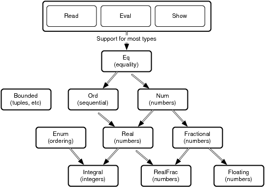
Figure 9. Important Haskell classes |
Classes do support inheritance, and it behaves like you think it should. For example, the Num class has subclasses Fractional and Real. Figure 9, Important Haskell classes shows the hierarchy of the most important Haskell classes in Haskell 98. Remember, instances of these classes are types, not data objects!
From the time I decided to write this book, I’ve dreaded writing the section on monads. After some study, I’ve learned that the concepts are not all that difficult. In this section, I’ll walk you through the intuitive description of why we need monads. Then, we’ll look at a high-level description of how monads are built. Finally, we’ll introduce some syntactic sugar that should really bring home how they work.
I leaned on a couple of tutorials to help shape my understanding. The Haskell wiki[27] has several good examples that I read, and also Understanding Monads[28] has some good practical examples. But you’ll probably find that you need to wade through several examples from many different sources to come to an understanding of what monads can do for you.
Let’s say you have a pirate making a treasure map. He’s drunk, so he picks up a known point and a known direction and makes his way to the treasure with a series of staggers and crawls. A stagger moves two steps, and a crawl moves one step. In an imperative language, you will have statements strung together sequentially, where v is the value that holds distance from the original point, like this:
def treasure_map(v)
|
|
v = stagger(v)
|
|
v = stagger(v)
|
|
v = crawl(v)
|
|
return( v )
|
|
end
|
We have several functions that we call within treasure_map that sequentially transform our state, the distance traveled. The problem is that we have mutable state. We could do the problem in a functional way, like this:
| haskell/drunken-pirate.hs | |
module Main where
|
|
|
|
stagger :: (Num t) => t -> t
|
|
stagger d = d + 2
|
|
crawl d = d + 1
|
|
|
|
treasureMap d =
|
|
crawl (
|
|
stagger (
|
|
stagger d))
|
|
You can see that the functional definition is inconvenient to read. Rather than stagger, stagger, and crawl, we must read crawl, stagger, and stagger, and the arguments are awkwardly placed. Instead, we’d like a strategy that will let us chain several functions together sequentially. We can use a let expression instead:
letTreasureMap (v, d) = let d1 = stagger d
|
|
d2 = stagger d1
|
|
d3 = crawl d2
|
|
in d3
|
Haskell allows us to chain let expressions together and express the final form in an in statement. You can see that this version is almost as unsatisfying as the first. The inputs and outputs are the same, so it should be easier to compose these kinds of functions. We would like to translate stagger(crawl(x)) into stagger(x) · crawl(x), where · is function composition. That’s a monad.
In short, a monad lets us compose functions in ways that have specific properties. In Haskell, we’ll use monads for several purposes. First, dealing with things such as I/O is difficult because in a pure functional language, a function should deliver the same results when given the same inputs, but for I/O, you would want your functions to change based on the state of the contents of a file, for example.
Also, code like the drunken pirate earlier works because it preserves state. Monads let you simulate program state. Haskell provides a special syntax, called do syntax, to allow programs in the imperative style. Do syntax depends on monads to work.
Finally, something as simple as an error condition is difficult because the type of thing returned is different based on whether the function was successful. Haskell provides the Maybe monad for this purpose. Let’s dig a little deeper.
At its basic level, a monad has three basic things:
A type constructor that’s based on some type of container. The container could be a simple variable, a list, or anything that can hold a value. We will use the container to hold a function. The container you choose will vary based on what you want your monad to do.
A function called return that wraps up a function and puts it in the container. The name will make sense later, when we move into do notation. Just remember that return wraps up a function into a monad.
A bind function called >>= that unwraps a function. We’ll use bind to chain functions together.
All monads will need to satisfy three rules. I’ll mention them briefly here. For some monad m, some function f, and some value x:
You should be able to use a type constructor to create a monad that will work with some type that can hold a value.
You should be able to unwrap and wrap values without loss of information. (monad >>= return = monad)
Nesting bind functions should be the same as calling them sequentially. ((m >>= f) >>= g = m >>= (\x -> f x >>= g))
We won’t spend a lot of time on these laws, but the reasons are pretty simple. They allow many useful transformations without losing information. If you really want to dive in, I’ll try to leave you plenty of references.
Enough of the theory. Let’s build a simple monad. We’ll build one from scratch, and then I’ll close the chapter with a few useful monads.
The first thing we’ll need is a type constructor. Our monad will have a function and a value, like this:
| haskell/drunken-monad.hs | |
module Main where
|
|
data Position t = Position t deriving (Show)
|
|
|
|
stagger (Position d) = Position (d + 2)
|
|
crawl (Position d) = Position (d + 1)
|
|
|
|
rtn x = x
|
|
x >>== f = f x
|
|
The three main elements of a monad were a type container, a return, and a bind. Our monad is the simplest possible. The type container is a simple type constructor that looks like data Position t = Position t. All it does is define a basic type, based on an arbitrary type template. Next, we need a return that wraps up a function as a value. Since our monad is so simple, we just have to return the value of the monad itself, and it’s wrapped up appropriately, with (rtn x = x). Finally, we needed a bind that allows us to compose functions. Ours is called >>==, and we define it to just call the associated function with the value in the monad (x >>== f = f x). We’re using >>== and rtn instead of >>= and return to prevent collisions with Haskell’s built-in monad functions.
Notice that we also rewrote stagger and crawl to use our homegrown monad instead of naked integers. We can take our monad out for a test-drive. Remember, we were after a syntax that translates from nesting to composition. The revised treasure map looks like this:
treasureMap pos = pos >>==
|
|
stagger >>==
|
|
stagger >>==
|
|
crawl >>==
|
|
rtn
|
And it works as expected:
*Main> treasureMap (Position 0)
|
|
Position 5
|
That syntax is much better, but you can easily imagine some syntactic sugar to improve it some more. Haskell’s do syntax does exactly that. The do syntax comes in handy especially for problems like I/O. In the following code, we read a line from the console and print out the same line in reverse, using do notation:
| haskell/io.hs | |
module Main where
|
|
tryIo = do putStr "Enter your name: " ;
|
|
line <- getLine ;
|
|
let { backwards = reverse line } ;
|
|
return ("Hello. Your name backwards is " ++ backwards)
|
|
Notice that the beginning of this program is a function declaration. Then, we use the simple do notation to give us the syntactic sugar around monads. That makes our program feel stateful and imperative, but we’re actually using monads. You’ll want to be aware of a few syntax rules.
Assignment uses <-. In GHCI, you must separate lines with semicolons and include the body of do expressions, and let expressions therein, within braces. If you have multiple lines, you should wrap your code in :{ and }: with each on a separate line. And now, you can finally see why we called our monad’s wrapping construct return. It neatly packages a return value in a tidy form that the do syntax can absorb. This code behaves as if it were in a stateful imperative language, but it’s using monads to manage the stateful interactions. All I/O is tightly encapsulated and must be captured using one of the I/O monads in a do block.
Every monad has an associated computational strategy. The identity monad, which we used in the drunken-monad example, just parrots back the thing you put into it. We used it to convert a nested program structure to a sequential program structure. Let’s take another example. Strange as it may seem, a list is also a monad, with return and bind (>>=) defined like this:
instance Monad [] where
|
|
m >>= f = concatMap f m
|
|
return x = [x]
|
Recall that a monad needs some container and a type constructor, a return method that wraps up a function, and a bind method that unwraps it. A monad is a class, and [] instantiates it, giving us our type constructor. We next need a function to wrap up a result as return.
For the list, we wrap up the function in the list. To unwrap it, our bind calls the function on every element of the list with map and then concatenates the results together. concat and map are applied in sequence often enough that there’s a function that does both for convenience, but we could have easily used concat (map f m).
To give you a feel for the list monad in action, take a look at the following script, in do notation:
Main> let cartesian (xs,ys) = do x <- xs; y <- ys; return (x,y)
|
|
Main> cartesian ([1..2], [3..4])
|
|
[(1,3),(1,4),(2,3),(2,4)]
|
We created a simple function with do notation and monads. We took x from a list of xs, and we took y from a list of xy. Then, we returned each combination of x and y. From that point, a password cracker is easy.
| haskell/password.hs | |
module Main where
|
|
crack = do x <- ['a'..'c'] ; y <- ['a'..'c'] ; z <- ['a'..'c'] ;
|
|
let { password = [x, y, z] } ;
|
|
if attempt password
|
|
then return (password, True)
|
|
else return (password, False)
|
|
|
|
attempt pw = if pw == "cab" then True else False
|
|
Here, we’re using the list monad to compute all possible combinations. Notice that in this context, x <- [lst] means “for each x taken from [lst].” We let Haskell do the heavy lifting. At that point, all you need to do is try each password. Our password is hard-coded into the attempt function. There are many computational strategies that we could have used to solve this problem such as list comprehensions, but this problem showed the computational strategy behind list monads.
So far, we’ve seen the Identity monad and the List monad. With the latter, we learned that monads supported a central computational strategy. In this section, we’ll look at the Maybe monad. We’ll use this one to handle a common programming problem: some functions might fail. You might think we’re talking about the realm of databases and communications, but other far simpler APIs often need to support the idea of failure. Think a string search that returns the index of a string. If the string is present, the return type is an Integer. Otherwise, the type is Nothing.
Stringing together such computations is tedious. Let’s say you have a function that is parsing a web page. You want the HTML page, the body within that page, and the first paragraph within that body. You want to code functions that have signatures that look something like this:
paragraph XmlDoc -> XmlDoc
|
|
...
|
|
|
|
body XmlDoc -> XmlDoc
|
|
...
|
|
|
|
html XmlDoc -> XmlDoc
|
|
...
|
They will support a function that looks something like this:
paragraph body (html doc)
|
The problem is that the paragraph, body, and html functions can fail, so you need to allow a type that may be Nothing. Haskell has such a type, called Just. Just x can wrap Nothing, or some type, like this:
Prelude> Just "some string"
|
|
Just "some string"
|
|
Prelude> Just Nothing
|
|
Just Nothing
|
You can strip off the Just with pattern matching. So, getting back to our example, the paragraph, body, and html documents can return Just XmlDoc. Then, you could use the Haskell case statement (which works like the Erlang case statement) and pattern matching to give you something like this:
case (html doc) of
|
|
Nothing -> Nothing
|
|
Just x -> case body x of
|
|
Nothing -> Nothing
|
|
Just y -> paragraph 2 y
|
And that result is deeply unsatisfying, considering we wanted to code paragraph 2 body (html doc). What we really need is the Maybe monad. Here’s the definition:
data Maybe a = Nothing | Just a
|
|
|
|
instance Monad Maybe where
|
|
return = Just
|
|
Nothing >>= f = Nothing
|
|
(Just x) >>= f = f x
|
|
|
|
...
|
The type we’re wrapping is a type constructor that is Maybe a. That type can wrap Nothing or Just a.
return is easy. It just wraps the result in Just. The bind is also easy. For Nothing, it returns a function returning Nothing. For Just x, it returns a function returning x. Either will be wrapped by the return. Now, you can chain together these operations easily:
Just someWebPage >>= html >>= body >>= paragraph >>= return
|
So, we can combine the elements flawlessly. It works because the monad takes care of the decision making through the functions that we compose.
In this section, we took on three demanding concepts: Haskell types, classes, and monads. We started with types, by looking at the inferred types of existing functions, numbers, booleans, and characters. We then moved on to some user-defined types. As a basic example, we used types to define playing cards made up of suits and ranks for playing cards. We learned how to parameterize types and even use recursive type definitions.
Then, we wrapped up the language with a discussion of monads. Since Haskell is a purely functional language, it can be difficult to express problems in an imperative style or accumulate state as a program executes. Haskell’s designers leaned on monads to solve both problems. A monad is a type constructor with a few functions to wrap up functions and chain them together. You can combine monads with different type containers to allow different kinds of computational strategies. We used monads to provide a more natural imperative style for our program and to process multiple possibilities.
Find:
A few monad tutorials
A list of the monads in Haskell
Do:
Write a function that looks up a hash table value that uses the Maybe monad. Write a hash that stores other hashes, several levels deep. Use the Maybe monad to retrieve an element for a hash key several levels deep.
Represent a maze in Haskell. You’ll need a Maze type and a Node type, as well as a function to return a node given its coordinates. The node should have a list of exits to other nodes.
Use a List monad to solve the maze.
Implement a Monad in a nonfunctional language. (See the article series on monads in Ruby.[29])